Rapidity as a Decomposition and a Writing Exercise

Back in December I posted a picture of the poster that I was taking to the Dallas Astrophysics Symposium. Lots of people asked what it all meant and I promised I’d answer eventually. Well, I've finally found the time to at start expanding on the poster in small chunks. The following is a first attempt and will make far more sense to physicists than it will to anyone else, (at least I hope it’ll make sense to someone).. I’m using these posts as a practice ground for explaining these concepts simply and the explanations should get better as time progresses. In the meantime, thanks for being my practice audience if you decide to read this! If you have questions, please ask them, and if you can see an obviously better way of expressing the ideas, and you’d like to share it that would be awesome and help a lot!

Physicists in the early 1900s defined a quantity called rapidity that serves as a way of measuring how fast a particle is traveling in special relativistic terms. Rapidity itself isn't a velocity, but it can be converted into the velocity of the particle as measured in the laboratory frame using the expression on the first line of picture one below. In the expression, the rapidity is denoted as w. The v to the left of the equal sign denotes the velocity of a particle as measured in the laboratory.

If we rearrange the expression a little bit, we get the second line in the first picture. Then, if we graph the right hand side of the equation, we get picture two. If you take a look, you’ll see that the velocity as measured in the laboratory never gets larger than the speed of light no matter how large the rapidity is. That's kind of nice since it fits with what the theory of special relativity tells us: the velocity of a particle measured in the laboratory frame never exceeds the speed of light.

The hyperbolic trigonometric functions follow similar rules to the more familiar circular trigonometric functions, so I can rewrite the expression in the first picture in the manner shown below in the first line of picture three.

Once I've done that, I can point out that the denominator is actually the ratio of how much time progresses in the lab per time as perceived by the moving particle. This ratio is associated with time dilation. If we look at a graph of the hyperbolic cosine, (picture 4), we see that the ratio can never be less than one and that it can become infinitely large.

Incidentally, the graph shown in picture four in geometric terms is called a catenary. It looks a lot like a parabola, but its not. Catenaries come up frequently in physics and are very interesting in their own right, but I digress, (they’ll turn up again later though… I promise). What this graph tells us is that if we stand still, (have a rapidity of zero), then our time ticks off at the same rate as time in the laboratory. However if we begin to move, even a little bit, laboratory time will tick off more quickly than the time we measure sitting on our moving particle.

The numerator of the expression in picture three is the rate at which distance traveled in the laboratory changes with respect to time as measured on the moving particle. There’s a really interesting point to be made here. Look at the graph of sinh in picture five. You’ll see that as w increases, the graph moves upwards towards infinity.

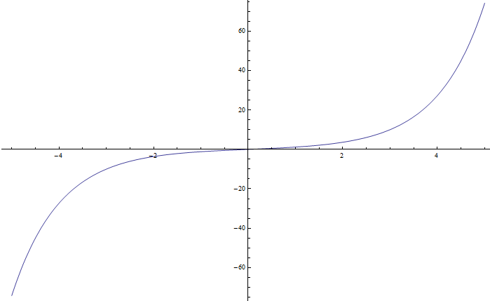
While we can’t measure a velocity faster than the speed of light in the laboratory, (see the left hand side of the expression in picture one), but if we measure distance traveled in the laboratory from the perspective of the particle, the result can be as much faster than the speed of light as we please! Does this violate the theory of special relativity? Nope! Special relativity merely says that we can’t measure the speed of a particle in the laboratory to be faster than the velocity of light. Have we known about this right from the start? Yup! If you have access to a university library check out the article by Wolfgang Rindler referenced below where he calculates how many light years a traveler could cover in an average lifetime. The quick answer is “many more light years than the years in the lifetime of the traveler”.

References
1. http://dx.doi.org/10.1103%2FPhysRev.119.2082
Rindler W. (1960). Hyperbolic Motion in Curved Space Time, Physical Review, 119 (6) 2082-2089. DOI: 10.1103/PhysRev.119.2082

2. Special Relativity by Wolfgang Rindler
http://books.google.com/books?id=8kqBAAAAIAAJ

3. On four velocity

http://copaseticflow.blogspot.com/2013/02/spheres-special-relativity-and-rotations.html

4. Poster post

More Cowbell! Record Production using Google Forms and Charts

First, the what : This article shows how to embed a new Google Form into any web page. To demonstrate ths, a chart and form that allow blog readers to control the recording levels of each instrument in Blue Oyster Cult's "(Don't Fear) The Reaper" is used. HTML code from the Google version of the form included on this page is shown and the parts that need to be modified are highlighted. Next, the why : Google recently released an e-mail form feature that allows users of Google Documents to create an e-mail a form that automatically places each user's input into an associated spreadsheet. As it turns out, with a little bit of work, the forms that are created by Google Docs can be embedded into any web page. Now, The Goods: Click on the instrument you want turned up, click the submit button and then refresh the page. Through the magic of Google Forms as soon as you click on submit and refresh this web page, the data chart will update immediately. Turn up the:

Cool Math Tricks: Deriving the Divergence, (Del or Nabla) into New (Cylindrical) Coordinate Systems

Now available as a Kindle ebook for 99 cents ! Get a spiffy ebook, and fund more physics The following is a pretty lengthy procedure, but converting the divergence, (nabla, del) operator between coordinate systems comes up pretty often. While there are tables for converting between common coordinate systems , there seem to be fewer explanations of the procedure for deriving the conversion, so here goes! What do we actually want? To convert the Cartesian nabla to the nabla for another coordinate system, say… cylindrical coordinates. What we’ll need: 1. The Cartesian Nabla: 2. A set of equations relating the Cartesian coordinates to cylindrical coordinates: 3. A set of equations relating the Cartesian basis vectors to the basis vectors of the new coordinate system: How to do it: Use the chain rule for differentiation to convert the derivatives with respect to the Cartesian variables to derivatives with respect to the cylindrical variables. The chain

The Valentine's Day Magnetic Monopole

There's an assymetry to the form of the two Maxwell's equations shown in picture 1. While the divergence of the electric field is proportional to the electric charge density at a given point, the divergence of the magnetic field is equal to zero. This is typically explained in the following way. While we know that electrons, the fundamental electric charge carriers exist, evidence seems to indicate that magnetic monopoles, the particles that would carry magnetic 'charge', either don't exist, or, the energies required to create them are so high that they are exceedingly rare. That doesn't stop us from looking for them though! Keeping with the theme of Fairbank[1] and his academic progeny over the semester break, today's post is about the discovery of a magnetic monopole candidate event by one of the Fairbank's graduate students, Blas Cabrera[2]. Cabrera was utilizing a loop type of magnetic monopole detector. Its operation is in concept very sim

Copasetic Flow

Search This Blog